Summer Researcher with Dr. Sarah Dodson-Robinson
Physics (Astronomy Concentration), Mathematics
University of Delaware
Maeve’s Research Summary:
In the research I took part in this summer, we were looking for exoplanets via data from a star’s spectra. First, I worked towards understanding the physics behind the data we had to analyze. Next we had to find the signals within the data, then we used statistical methods to confirm that the signals were actually planets and weren’t just stellar activity. Stellar activity (ie. solar flares, sun spots, etc) typically occurs because the convective layers in the star interact with its magnetic field, causing fluctuations in the star’s emitted light which affects its spectrum. Within this project, my specific role
was to further analyze published findings of planets by generating power spectrum estimates (e.g. VanderPlas 2018) as well as Magnitude squared coherence (Dodson-Robinson et al. 2022) for radial velocity and stellar indicator measurements in the data. These published data sets do not include magnitude squared coherence
measurements in the data, so further investigation is necessary to validate or question these findings.
A star being orbited by a planet is not the full picture of what is happening in the system. The star and the planet orbit around a shared center of mass which is usually somewhere within the star (along its radius), but not exactly in the center of the star. Physically, this principle is seen by the star’s “wobble” about this center of mass. Stars are constantly emitting photons in the form of a unique spectrum that depends on its chemical composition and temperature. Due to the Doppler effect, particular wavelengths in the spectra shift when the star moves radially towards or away from the
observer in their line of sight. Using the doppler equation and the measured shift of the wavelength lines, the radial velocity of the star can be calculated. For a particular star, astronomers on Earth take multiple data recordings on radial velocity measurements and
activity indicators (which will be discussed later) of the star. These points are taken simultaneously for all radial velocities and indicators and are taken incrementally over long periods of time, sometimes many years.
The other data that astronomers collect are activity indicators such as S-index on the Mt. Wilson scale, Line Bisector/span bisector, Full width at half maximum and H-alpha. It is important to analyze these indicators alongside the radial velocity data because in a spectrum, the doppler shift due to radial velocity shifts all wavelengths, while activity such as sunspots or flares for example are only present at specific wavelengths because unlike the orbit of a planet, they are typically not cyclical events. The S-index indicator analyzes two different absorption lines centered on calcium emission cores and takes a ratio of these lines to the continuum regions on either side of
these lines. Line bisector measures the velocity location of the midpoint between the spectral line of the core (center) to that of the continuum. Full width at half maximum measures the width of an absorption where the amplitude is at half the maximum amplitude.
We create plots called power spectra or periodograms that give a representation of a time series (data indexed in time order) in terms of wave power at different frequencies, so that we can see at which frequencies there are statistically significant peaks in power. In our research we plotted Lomb-Scargle periodograms as well as Welch’s power spectrum estimates which have cleaner spectral windows (less noise in the data). Based on the power of the amplitude, we can determine whether the peaks in the data are significant (represent a signal) or not (represent white noise in the data). Statistically, we are testing to see if we should reject or fail to reject a null hypothesis.
- Null hypothesis: the data set is just white noise
- Alternative hypothesis: there is at least one periodicity within the time series
To determine whether or not the peaks in the radial velocity data are caused by planets or by stellar activity, we used the statistical method called Magnitude squared coherence: a bivariate statistical technique used to plot the frequencies where both time series may trace the same physical process. When each coherence plot is made
between a radial velocity set and indicator, the amplitude of the coherence is recorded at various frequencies. Peaks in this data set indicate that at that particular frequency, the two series overlap, and therefore the peak in the radial velocity could be just stellar activity manifesting in the data. If the frequency at which there is high coherence is located on the frequency of a potential planet candidate, this would indicate that it could be a false positive.
The first data set I analyzed was GJ 625, a small red dwarf star with a planet detected with an orbital period of about 14 days (Suarez Mascareno et al. 2017). Using a python notebook and NWelch program (Dodson-Robinson 2022), first the data (consisting of the Julian date of the observation and each corresponding radial velocity
(RV) measurement and indicator) was read in. Each variable was plotted at a scatter plot, a frequency grid was developed, the data was put into multiple shorter segments, and both a Lomb-Scargle and Welch’s power spectrum estimate were generated. On the spectrum estimate plots, the planet’s orbital frequency and star’s rotational frequency were both plotted as vertical dotted lines, and the false alarm levels (5%, 1%, 0.1%) were plotted as horizontal lines. There were significant signals at the reported rotation frequency as well as the 2nd and 8th rotational harmonics in the H-alpha index for the LS periodogram, but the power of these signals greatly diminished when plotted using the Welch algorithm. This can also be seen using statistical Siegel tests on each periodogram, where the null hypothesis is that the data is just white noise and the alternative hypothesis is that there are significant periodicities detected in the data. For the Lomb-Scargle periodogram, the null hypothesis was rejected, whereas in Welch’s periodogram, the null hypothesis failed to be rejected. Lastly, we can visualize the spectral window in which the data was recorded. For this star, the only other index in which the rotation had a significant peak for the Welch’s power spectrum estimate was in the Full width at half maximum (FWHM), where the peak near the planet frequency was well above the 0.1% bootstrap level. The S-index on the Mount Wilson scale (SMW) had a peak just under the 5% level, and Bisector Span was completely white noise. When the RV data were plotted, the planet’s orbital frequency was plotted as a vertical line and there were peaks, but they did not rise above the 5% FAP, meaning that further investigation should be done to determine whether the detected planet is true or is really
just a stellar signal manifesting in the data.
In the second notebook for this star, the Magnitude Squared coherence between each radial velocity measurement and activity indicator were calculated and plotted. For each pair, a bivariate object is created (a total of 8 objects) to make coherence graphs
and determine if there are peaks around the detected “planet”, meaning that at this frequency there is significance similarity in the power of the activity indicator which could then be accounting for the “planet’s” signature. The only significant peak in coherence
was in the RV-CCF x FWHM plot on the planet which was above the 1% FAP.
The next task was to analyze the data from a similar M-type star GJ 667C, a member of a trinary system with 7 reported potential planet discoveries (Feng et al. 2017). I analyzed 6 because the 7th was not reported confidently in the literature. The data set consisted of RV-Terra and RV-CCF, FWHM, S-index and bisector span. In both the FWHM and SMW scatter plots, there was 1 point in each data set that was an outlier. I analyzed the periodogram of the full data set and compared this to a data set that excluded this point (clipped) and found that the power of all periodogram peaks decreased when excluding the point. Outlying data can affect the overall powers, leading to false positives. In both RV periodograms, the planet b signal had very high power, while the other 5 signals had small, yet noticeable peaks (figure 1). According to the Siegle tests conducted, both RVs, FWHM and FWHM-clipped had significant periodicities, while the bisector span and S-index was determined to be white noise, and the S-index-clipped set had a peak at rotational frequency, though not very significant.
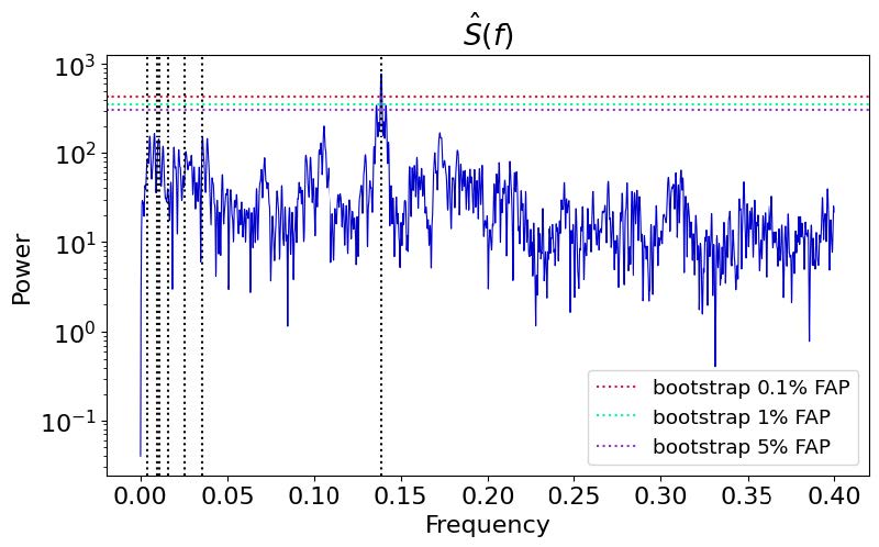
the power of the rightmost signal (planet b) is well above the 0.1% false alarm level.
Overall, when computing the magnitude squared coherence, planet b did not have any significant coherence with any of the stellar indicators. There were less peaks in the clipped data than the regular data for SMW and FWHM, showing greater accuracy. There was a strong coherence peak on planet d’s frequency for SMW-unclipped and RV-Terra, which migrated to the rotational frequency in the clipped version. This should be followed up with, because the physical processes that caused the outlier from the data (that was clipped out) could be responsible for the signal interpreted as planet d. Planet e had a peak on the 1% FAP for RV-CCF x FWHM-clipped. Planet d had a high coherence for SMW-unclipped and RV-CCF, which when clipped, did not surpass the 1% bootstrap level. (See figure 2 below for an example of a transformed magnitude squared
coherence plot).
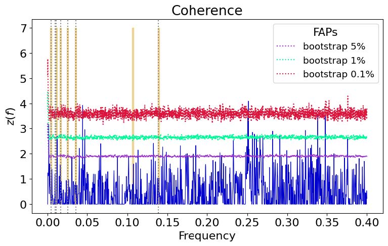
Note that there are no significant coherence peaks on any of the vertical dotted lines that represent planets.
Furthermore, white noise data experiments in which coherence measurements are created between sets of random data points and each RV, FWHM-clipped and SMW-clipped. For each variable, an array consisting of 10,000 rows of different coherence measurements at each frequency grid increment was created and plotted. Three histograms were plotted for each threshold with counts of number of crossings and bins of frequency. There were consistent high peaks at the zero frequency for all sets. For RV-Terra, there were high peaks around planets c and f. These planets also had noticeable yet insignificant peaks for FWHM. The random data x random data
yielded no counts of crossings at the 0.1% significance level. Overall, no strong peaks stood out around planet signals for this experiment, potentially indicating that the signals in the literature could be verified, but more research is needed. Forthcoming, further analysis of the 5 lower frequency signals should be done excluding planet b so that the overall power is adjusted and the significance of the peaks can be determined.
I really enjoyed working with Dr. Dodson-Robinson as well as the team of graduate students and my undergraduate peers. Team meetings kept us on track and allowed the undergraduates to present our findings as well as receive feedback from and ask questions of experienced researchers. This experience improved my understanding of statistical analysis, coding (python), graph analysis and the physics behind searching for exoplanets (especially how data is collected by terrestrial telescopes). It also provided a valuable glimpse into what is required of graduate students who wish to pursue a PhD, and of a research professional in the astrophysics field.