
Summer Researcher with Dr. Sarah Dodson-Robinson
Physics, Concentration in Astronomy and Astrophysics
University of Delaware
Allison’s Research Summary:
Introduction
This summer I worked with Sarah Dodson-Robinson on detecting exoplanets which are planets outside of the solar system from signals in a star’s spectra. The main goal was to confirm if a signal was actually a planet or the star’s activity. Every star constantly emits photons, or light in it’s own unique spectrum that is dependent on the star’s composition and temperature.

lines occur when photons are absorbed by gas as they are traveling to the observer
on Earth.
A planet orbiting a star follows Newton’s law of universal gravitation:
The star is represented by mass m1 and the planet is represented by m2 and they both orbit around a shared center of mass. The center of mass is closest to the more massive object, in this case that would be the star. As the planet moves around the star it causes the star to ”wobble”. Due to this wobble, it causes the star’s spectrum to shift because of the Doppler effect. On Earth we can observe these shifts in the absorption lines and measure the radial velocity of the star. Through this data we can confirm if a planet is present in the system.
However, stellar activity can mask the radial velocity signals or get mistaken for signals, making it more difficult to detect planets. Multiple measurements of different activity indicators of the star must be taken to further validate radial velocity measurements. The activity indicators measured are hα, S-index, bisector span, and full width at half maximum. Hα is a deep red spectral line that is emitted when a hydrogen atom’s electron falls from the third energy state to the second. S-index is calculated by taking a ratio of two absorption
lines to the entire spectrum region. This helps show the magnetic activity of the star. For example, a larger ratio signifies more variability in the magnetic field. The bisector span shows the skew of the star’s spectral lines. The more skew, the more activity the star has. Lastly, the full width half maximum is the midpoint of the minimum of the average shape of the spectral lines. This measures the speed of gasses in the star’s chromosphere or upper atmosphere.
Analysis
The star I analysed is GJ 625 which is a red dwarf located 21.1 light years from the sun based on parallax. In 2017 a planet was detecting orbiting the star with a period of 14.7 days. To further test the validity of the detection I used Sarah Dodson-Robinson’s NWelch software. I began with taking a Fourier transform of the data to find which wave frequencies are present. A Fourier transform breaks down complex mathematical functions into sums of sines and cosines. By taking the square of the absolute value of the Fourier transformed function, power spectrum/periodogram plots can be made. A Lomb-Scargle periodogram is a least squares spectral analysis for the time series of velocity measurements. A time series is a set of data points indexed in order of time. Welch’s power spectrum is also a periodogram but has a cleaner spectral window which improves the ability to estimate planet rotation speeds.
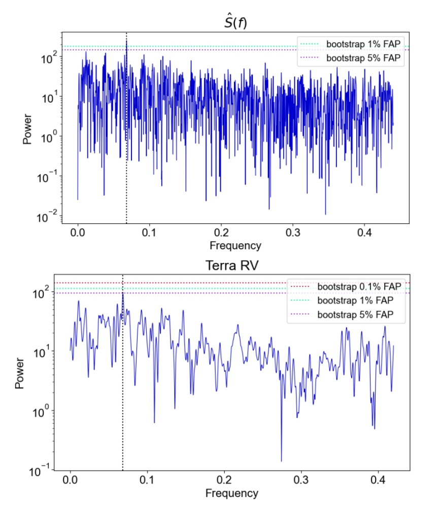
(a) Lomb-Scargle periodogram of radial velocity calculated by the Terra pipeline.
(b) Welch’s power spectrum of the Terra calculated radial velocity. The dotted black line represents the detected planet. The 3 horizontal lines are false alarm probabilities. For example, if a line passes over the one percent false probability line there is a 99 percent chance that the signal is a planet.
The next step was to plot a magnitude squared coherence which is a statistical technique used to plot frequencies where two time series have oscillations in common. When plotting the coherence of radial velocity to an activity indicator it is important to notice if there are peaks at or near the planet candidate’s orbital frequency. A shared signal may indicate that the signal is coming purely from stellar activity and may not be a planet signal. In the case of GJ 625, there were some large peaks at or near the planet’s orbital frequency on about half of the coherence plots. This raised some concerns that stellar activity was acting as a planetary signal and further analysis was needed.
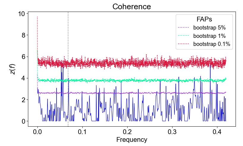
velocity calculated by the cross correlation function (CCF) and full width half
maximum. There is a peak on the black dotted line that signifies the planet’s
frequency that crosses about the one percent false alarm probability. Similar
trends occurred on several coherence plots.
To further test if there was a possible false positive planet detection I made two sets of fake data. The fake data sets will essentially act as noise and will not have a trend. After plotting the magnitude squared coherence of the fake data sets to the Terra radial velocity and CCF radial velocity, peaks were still occurring at or very close to the planet’s frequency. This may indicate an anomaly at a particular frequency.
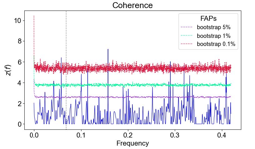
set to Terra radial velocity. The large peak in coherence is very close to the
planet’s frequency and very similar trends occur when plotting the coherence of
other fake data sets to radial velocity.
Finally, to pinpoint any frequencies that may be causing an anomaly in the data I created ten thousand iterations of fake data and plotted the coherence of iterations to all the activity indicators and previously created fake data sets. To really pinpoint a particular frequency I plotted histograms of the amount of times the iterations crossed over each false alarm threshold at each frequency. On all the plots the only large amount of crossings occurred at the zero frequency which doesn’t have any significance.
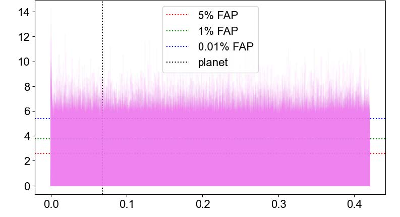
of random data to Terra radial velocity. The opacity of each line plotted was
set to a very low value to see where majority of the data points fell. There is
a large peak observed at the zero frequency which does not raise any concerns
and was observed on the rest of magnitude squared coherence plots for all the
activity indicators. X-axis is frequency and Y-axis is z(f).
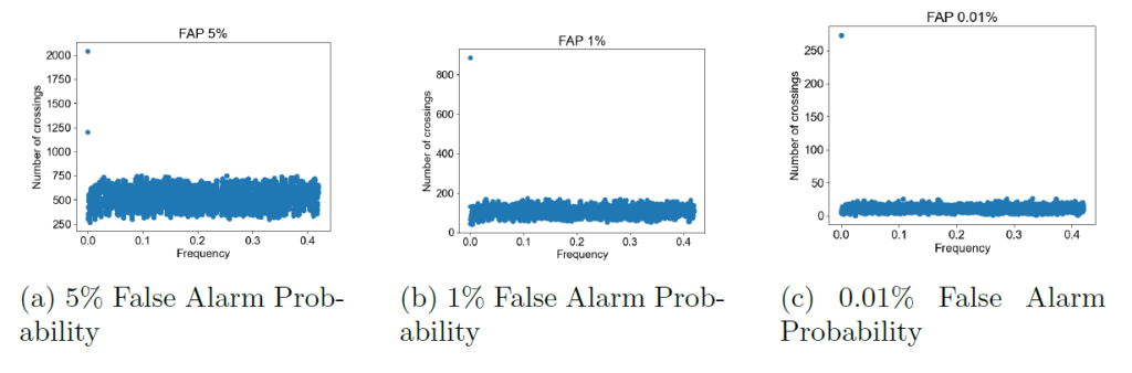
in the coherence plot showed in figure 5.
To also test if the times of observation influenced the results I did the same process with ten thousand iterations of random data and plotted Welch’s power spectrum. Observations can only occur at night and when the Earth is facing towards the star. Periods of time missing in observations could have an unwanted effect on the data. The ideal result would be a plot of a straight line but because no data set is perfect small fluctuations are expected. That pattern was observed in the plots that were produced and only small difference occurred once again showing that no frequencies were out of the ordinary.
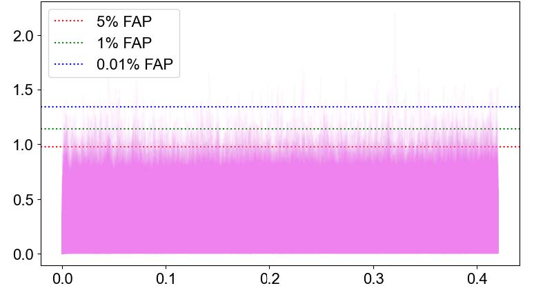
power spectrum. The X-axis is frequency and the Y-axis is power. There are
no significant variations to raise any concerns that observation timing affected
the data.
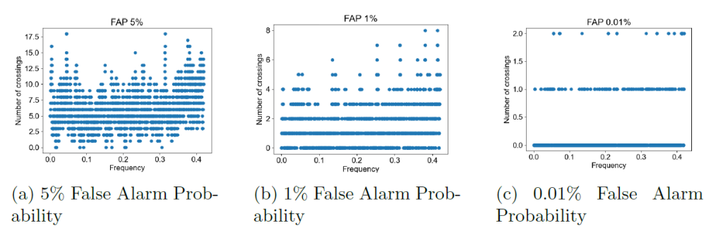
in the Welch’s power spectrum plot showed in figure 7.
Conclusion
Overall, the results of this experiment are ambiguous. More analysis would have to be done to be sure if this planet detection is a false positive. Since not all the magnitude squared coherence plots of the activity indicators to radial velocity had peaks at or near the planet’s frequency so it could possibly just be a coincidence. No frequencies seem to be contributing to anomalies in the data and observation timings also do not seem to be playing a part as well. It is important to be cautious when detecting planets based off radial velocity signals because a lot of factors could be contributing to the signal and false positives do occur.